Foundation models gesture at a way of interacting with information that’s at once more natural and powerful than “classic” knowledge tools. But to build the kind of rich, directly interactive information interfaces I imagine, current foundation models and embeddings are far too opaque to humans. Models and their raw outputs resist understanding. Even when we go to great lengths to try to surface what the model is “thinking” through black-box methods like prompting or dimensionality reduction approaches like PCA and UMAP, we can’t deliver interaction experiences that feel as direct and predictable, as “extension-of-self”, as multi-touch.
Solving this understandability gap is fundamental to unlocking richer interfaces to modern AI systems and the information they model. Good information interfaces open up not just new utility, but new understanding to users about their world, and without closing the understandability gap between frontier AI systems and humans, we can’t build good information interfaces with them.
This work explores a scalable, automated way to directly probe embedding vectors representing sentences in a small language model and “map out” what human-interpretable attributes are represented by specific directions in the model’s latent space. A human-legible map of models’ latent spaces opens doors to dramatically richer ways of interacting with information and foundation models, which I hope to explore in future research. In this work, I share two primitives that may be a part of such interfaces: detailed decomposition of concepts and styles in language and precise steering of high-level semantic text edits.
The bulk of this work took place between December 2023 and February 2024, concurrently with Anthropic’s application of similar methods on Claude Sonnet and OpenAI’s work on interpreting GPT-4, as a part of my research at Notion. I wrote this report at the end of February, and then subsequently came back to revise and add some updates in June 2024.
In this piece, I’ll use the words “latent space” and “embedding space” interchangeably; I use them to refer to the same entity in the models being studied.
Contents
- Key ideas
- Further motivations
- Demo
- Methodology
- Results and applications
- Caveats and limitations
- Future work
- Looking back, looking forward
- Appendix
Key ideas
Many of these are generalizations of findings in Anthropic’s sparse autoencoders work to text embeddings, alongside some new training and steering techniques.
-
Sparse autoencoders can discover tens of thousands of human-interpretable features in text embedding models.
Applying sparse autoencoders to text embeddings (with some training and architectural modifications), we’re able to recover tens of thousands of human-interpretable features from embedding spaces of size 512-2048.
Using this technique, we can:
- Get an intuitive sense of what kinds of features are most commonly represented by an embedding model over some dataset.
- Find the most strongly represented interpretable features for a given input. In other words, ask “What does the embedding model see in this span of text?”
- Answer “why” questions about embedding models’ outputs, like “Why are these two embeddings closer together than we’d expect?” or “How does adding a page title to this document affect the way the model encodes its meaning?”
For example, we can embed the title of this piece, Prism: mapping interpretable concepts and features in a latent space of language, and see that this activates features like “Starts with letter ‘P’”, “Technical discourse on formal logic and semantics”, “Language and linguistic studies”, “Discussion of features”, and “Descriptions of data analysis procedures”.
-
Interventions in latent space enable precise and coherent semantic edits to text that compose naturally.
Once we find meaningful directions in a model’s latent space, we can modify embeddings using this knowledge to make semantic edits, by pushing the embedding further in the direction of a specific feature. For example, we can turn a statement into a question using the “Interrogative sentence structure” feature without disrupting other semantics of the original text. Applying this edit to the title of this bullet point outputs:
“Insights into how can we make precise changes to the latent space’s text output?”
Semantic text editing works by modifying an embedding (in this case, via simple vector addition), then decoding it back into text using my Contra text autoencoder models.
This kind of precise semantic editing capability enables direct manipulation of models’ internal states as a way of interacting with information, as I first wrote about here in 2022.
I also share a novel way to make sparse autoencoder-based edits to embeddings I call feature gradients, which uses gradient descent at inference time to minimize interference between the desired feature and other unrelated features. This makes semantic edits in latent space even more precise than before. Furthermore, I demonstrate examples of multiple semantic edits using many different features stacking predictably to result in edits that express many different desired features at once, showing that edits in latent space can compose cleanly.
-
Large language models can automatically label and score its own explanations for features discovered with sparse autoencoders, and this process can be made much more efficient for a small sacrifice in accuracy with a new approach I call normalized aggregate scoring.
Building on OpenAI’s automated interpretability work, I propose a much more cost-efficient way to score a language model-written description of a sparse autoencoder feature that still appears to be well-aligned with human expectations.
This automated confidence score, a number between 0 and 1:
- Aligns with my human judgement of explanation quality. Specifically, the number of features with confidence greater than some threshold like 0.99, 0.9, or 0.75 are reliable predictors of overall quality of features in a particular SAE training run.
- Is precise enough to use as a part of hyperparameter search without human review of labels. This enabled me to do much more hyperparameter search than would have otherwise been possible as an individual researcher.
Further motivations
Beyond expanding the design space of rich information interfaces, there are several other reasons why interpretable embeddings are valuable.
Debugging & tuning embeddings
Embeddings are useful for clustering, classification, and search, but we usually treat embedding values as black boxes that give us no understanding of exactly why two inputs are similar, or what features of input data get encoded into embeddings.
This means when embeddings perform poorly, our debugging is less precise, and we aren’t able to express certain invariants about a problem like “we don’t care about the presence of punctuation or gendered pronouns” into queries involving embeddings.
If we understood how human-legible features were encoded in embeddings, we would be able to more precisely understand why embeddings underperform when they do, and perhaps allow us to manually tune embeddings quickly and cheaply with confidence.
Steerable text generation
When using AI for writing, current generation language models require the user to write in plain English exactly what edit they would like. But often, verbally specifying edits or preferences is laborious or impractical (e.g. when referring to a specific style of some sample text, or when trying to steer the model away from some common behavior).
In many graphics editing tools, rather than manually drawing shapes, users can use features like “copy style” to work more directly with stylistic elements of edits. They can even enumerate different elements of style (shape, color, shadow, border) and manually edit them with direct real-time feedback.
This work, especially if applied to more capable models, opens up ability for text editing tools to offer similar kinds of “direct style editing” features.
Demo
As of time of publication, I have a publicly hosted demo of everything in this work at https://linus.zone/prism.
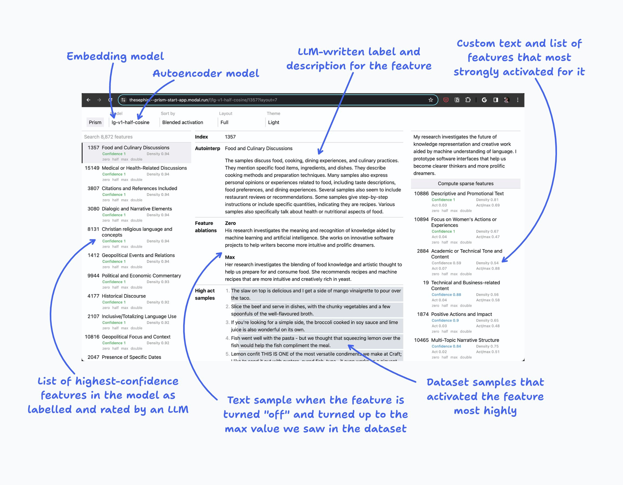
I built this as an internal research tool, so the interface isn’t the most intuitive, and there is some functionality I won’t explain here. But this is a quick overview of this tool:
-
Choose an embedding model and sparse autoencoder to study in the top left drop-down. I recommend starting with
lg-v6, which is a good balance of speed and expressiveness. In general, you should stick with the “v6” generation of sparse autoencoders.Each sparse autoencoder loads a new “dictionary” of features. For example,
lg-v6has around 8,000 features that it has extracted from the embedding space of thelargemodel found here, with a 1,024-dimensional embedding space. -
Select a feature in the left sidebar to see more information about that feature.
Index: index of this feature in the sparse autoencoder’s model weights. Not useful except as a unique ID.
Autointerp: GPT-4 written description of this feature, based on samples on which this feature activated strongly.
Feature edits: If the editor (described below) is open, this section shows semantically edited versions of the given text with the selected feature clamped to specific values.
High/low activation samples: Example sentences in the sparse autoencoder training dataset (currently a filtered subset of The Pile) that most strongly activated the feature, or did not activate the feature, respectively.
-
Enter some text into the right “Editor” sidebar and submit to see which features activate particularly strongly for that text.
Feature gallery
Here are some hand-curated interesting features I’ve found that represent the diversity of features discovered with this method.
Though I’ve spent a lot of time studying individual features in these datasets, I haven’t done any systematic dataset-wide study. So view these cherry-picked examples more as curious observations of what features look like, rather than a statement about the effectiveness of the specific techniques used or what the “typical” feature is.
Topic / subject matter
- Legal concepts and terminology
- References to cellular biology
- Railway and Train References
- Sweet Treats and Baking
- Discussion of astrophysical phenomena
- Agriculture and farming-related discussions
Sentiment and tone
Specific words or phrasing
- Starts with the letter ‘L’
- Beginning with ‘Despite’ indicating contrast
- Multi-geographic presence or operation, like “across five continents”
- Denied and confirmed assertions, as in the “not…, but…” rhetorical form
Punctuation, grammar, and structure of text
- First-person narrative quotes
- Comma-separated, descriptive adjective sequences, like “vibrant, brilliant, imaginative”
- Starts with special character, which turns out to be the prefix “- “, i.e. bulleted list items
- Presence of modal verbs “can” or “could”
- Consecutive statements linked with “and this”
Numbers, dates, counting
- Explicit mention of the number “two”
- Presence of the numbers 12 or 13
- Presence of ordered number sequences
Natural and code languages
- Written in French language
- Anime or Japanese game references
- JavaScript and jQuery code snippets
- Presence of web URLs
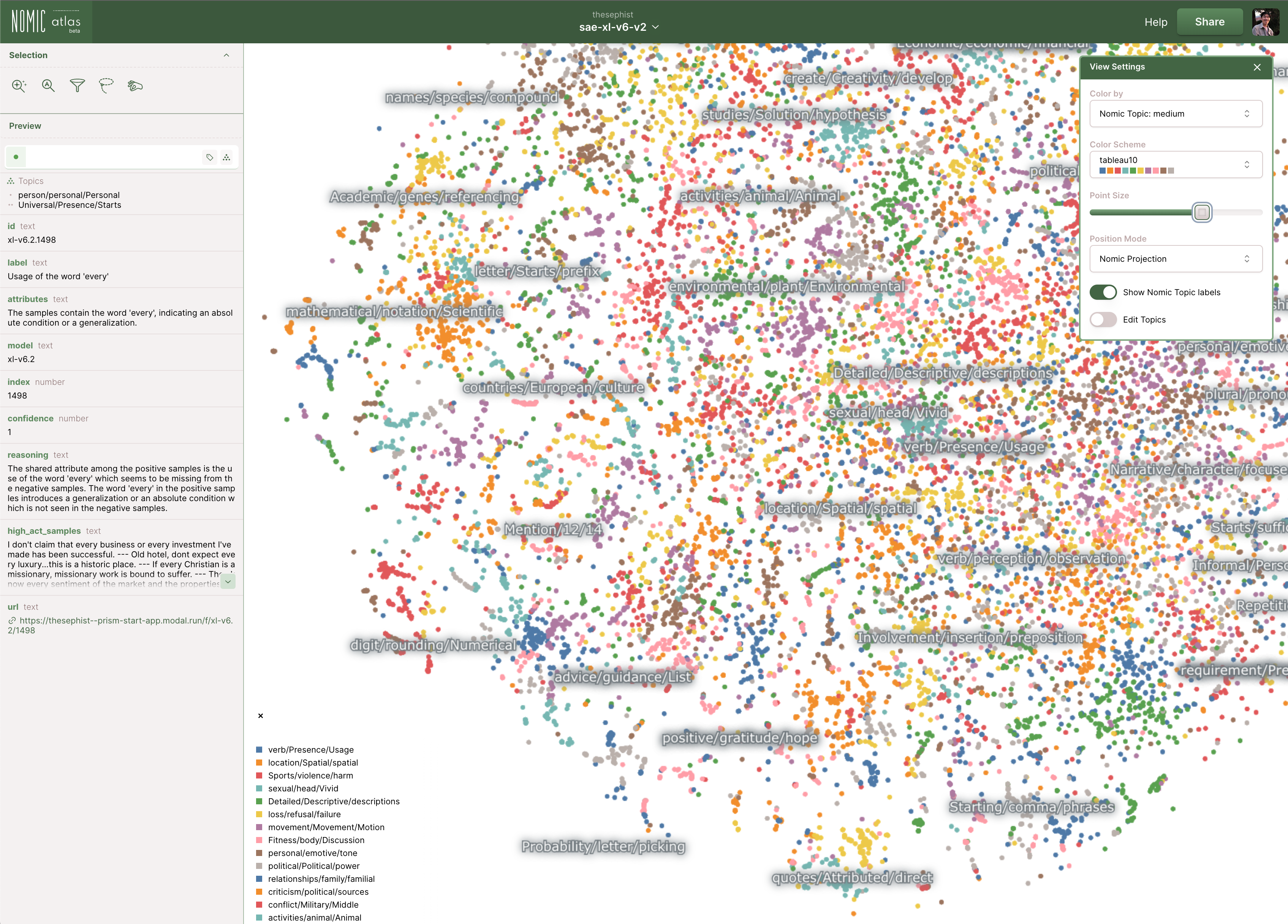
You can also visually explore every “confidently labelled” feature (confidence score above 0.8) in all trained v6 SAEs on Nomic Atlas, for sm-v6, bs-v6, lg-v6, and xl-v6. In these visualizations, each feature is represented by a dot and clustered nearby other features pointing in similar directions in embedding space.
Methodology
Sparse autoencoders draw on a rich history of mechanistic interpretability research, and to understand it in detail, we need to build a little intuition. If you’re versed in mech interp, feel free to skip ahead to the results.
Mechanistic interpretability as debugging models
One way to understand the goal of mechanistic interpretability is to think of a trained neural network as having learned a kind of program or algorithm. Neural networks learn numerous algorithms over the course of training, each of which accomplish a specific part of the network’s task. For example, a part of a neural net may implement an algorithm to know when to output a question mark, or an algorithm to look up specific facts about the world from its internal knowledge. As a model sees billions of samples of input during training, these algorithms slowly carve themselves into the model’s weight matrices, over time implementing a full program that excels at the tasks we train models to do, like predicting the next token in a string of text.
Interpreting a neural network, then, is a bit like trying to understand a big, complex program without any source code that explains its implementation.
Reverse engineering the algorithms in a neural network is a bit like reverse engineering a running black-box program. A program has variables which store specific values that represent something about the algorithm’s view of the world. These variables are computed from other variables by operations, like addition or multiplication, that connect these variables together. In a neural network, the variables are called features, and the operations are called circuits. For example, a language model may have a feature that represents whether a sentence is coming to an end, and a circuit that computes that feature’s value from other earlier features.
Just as a program combines simple primitive operations to form larger ones, a neural network is ultimately composed of millions and billions of features and circuits that connect to compute those features. To get a mechanistic understanding of how a model produces its outputs from its inputs, we need to be able to stick a debugger into the neural network’s internals, read out the values its features take on, and trace its circuits to understand how those features are computed from each other.
To establish some vocabulary:
- A feature is like a variable in a program. It’s a unit of meaning the model uses to represent something about its input.
- A circuit is some set of operations that compute a feature from earlier features, like operations or functions in a program.
- I’ll also sometimes refer to activations, or the values that features take on for a particular input. In a program, a variable called “width” may take on the value “300”. In a neural network, a feature for “positive sentiment” may take on the value, or activation, 0.5.
Background
Over the last few years, there’s been accelerating research into decomposing features within transformer models through a framework called dictionary learning, wherein we try to infer a “dictionary” of features that a model knows about. It’s a bit like trying to find a way to scan a black-box program and get all the variables inside it.
Notable prior art include:
- Transformer visualization via dictionary learning, Yun et al.
- Sparse Autoencoders Find Highly Interpretable Features in Language Models, Cunningham at al.
- Towards Monosemanticity: Decomposing Language Models With Dictionary Learning, Bricken et al. (Anthropic)
These approaches all build on the same core ideas:
-
Sparsity. While there are many concepts and features we care about in the space of all inputs, only a few features are relevant to each input. For example, any given sentence can only contain a handful of languages at most, and mention only a few people, while the model may know about hundreds of languages and thousands of famous people. We call this phenomenon, where each input only contains a small fraction of all known features, “sparsity”.
-
Superposition. A good model must learn potentially hundreds of thousands or millions of concepts, but may only have a few hundred dimensions in its latent space. To overcome this limitation, models learn to let features interfere with each other. In simple terms, this means the same direction may be re-used to represent multiple different directions, so long as they rarely occur together, and thus are unlikely to be confused for one another. For example, a model may choose to put “talks about cooking” and “memory allocation in C++” next to each other in latent space because only one of those features is likely relevant for any specific input. The model is taking advantage of sparsity to pack in more information into a smaller latent space.
Here’s a more technical rephrasing: within an embedding space of $n$ dimensions, good embedding models often compress many more $m \gg n$ features such that features that don’t often occur together are allowed to share directions and interfere with each other. Superposition becomes exponentially more effective as dimensionality increases. This allows models to represent far more features than it has dimensions, and is called the superposition hypothesis.
-
Autoencoding. To recover which features are compressed into a particular embedding space, we can train a secondary model to learn to represent the original model’s embeddings (in a process called “autoencoding”), but sparsely within a much larger latent space. In other words, this sparse autoencoder (SAE) model’s task is to find a way to pull apart the many, many features that were all packed into the original subject model’s latent space. The sparse autoencoder is trained to approximate the much larger, more sparse space of features, and then learn to map embeddings into and out of this larger, more sparse space.
Recent work from Cunningham et al. and Bricken et al. show this works reasonably well for small language models, recovering features like “this text is written in Arabic” or “this token is a part of a base64 string”. This work generalizes some of these findings to much larger text embedding models that are close to production scale.
In particular, Anthropic’s extremely detailed research report goes into fantastically helpful detail about their sparse autoencoder training recipe, including hyperparameter choices and architectures that did not work as well. These were tremendously helpful in my own experiments.
Training sparse autoencoders
Here, I share the concrete architecture and training recipes for my sparse autoencoders, including all the technical details. If you aren’t interested in digging into the specifics, feel free to skip down to the “Automated interpretability” section right below this one.
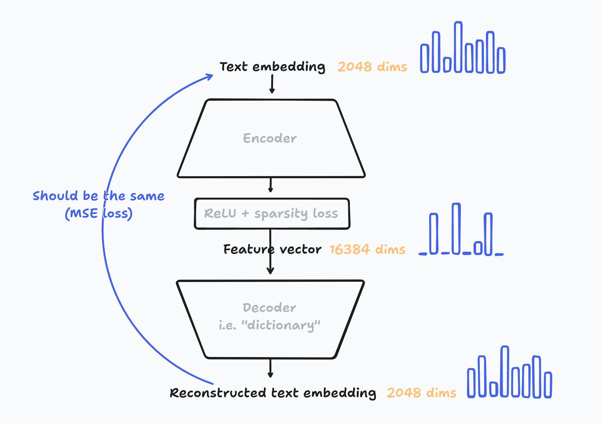
Below is a high-level concept diagram of how these sparse autoencoders are trained. The numbers in the illustration are for the xl-v6 SAE.
First, I take a medium size English language modeling dataset. Here, it’s Minipile. I chunk every data sample on sentence boundaries with nltk , giving me roughly 31M English sentences.
Then, I run each sentence through an embedding model (Contra) to generate 31M embeddings.
On this dataset of embeddings, I train a SAE that tries to learn a dictionary that’s 8x, 16x, 32x, and 64x larger than the size of the original embedding.
More specifically, my SAE closely follows architecture choices from Bricken et al.:
$$\mathbf{f} = \mathrm{ReLU}(W_e (\mathbf{x} - \mathbf{b}_d) + \mathbf{b}_e)$$
$$\hat{\mathbf{x}} = W_d \mathbf{f} + \mathbf{b}_d$$
$$\mathcal{L} = \frac{1}{|X|}\sum_{\mathbf{x} \in X}||\mathbf{x} - \hat{\mathbf{x}}||^2_2 + \lambda||\mathbf{f}||_1$$
Here,
- $\mathbf{x}$ and $\hat{\mathbf{x}}$ are input (original) and output (reconstructed) embeddings, respectively;
- $\mathbf{f}$ is the vector of activation values for every feature;
- $W_e$ and $W_d$ are encoder and decoder weights, respectively; and $\mathbf{b}_e$ and $\mathbf{b}_d$ are encoder and decoder biases, respectively;
- The loss $\mathcal{L}$ has two terms:
- Reconstruction loss, which measures the squared error between the reconstructed and original embeddings, and
- Sparsity loss, which is scaled by a hyperparameter $\lambda$ and pushes the feature space to be sparse.
In other words, my SAE is a two-layer model with the ReLU activation and a hidden layer size that’s 8, 16, 32, or 64x larger than the inputs and outputs.
Some more notes I made in my experiments about training:
- When using a high sparsity coefficient $\lambda$ with the default PyTorch weight initialization, it’s easy to accidentally “kill” (push to never activate) too many features early in training. I could effectively prevent this from happening by scaling the coefficient $\lambda$ from 0 to its full value over the first 1/4 of training steps.
- I did not use resampling (first noted by Anthropic) in the beginning to keep implementation simple, and later adopted Anthropic’s Ghost Grads and saw meaningful improvements. I also adopted their recommendation (corroborated by DeepMind’s alignment team) of setting the Adam optimizer’s $\beta_1$ hyperparameter to 0.
- Cunningham et al. uses a novel orthogonal weight initialization for the autoencoder, but Anthropic’s work seems to do fine with PyTorch’s default Kaiming init, and this is what I did as well.
In addition to loss and sparsity, the most reliable sign I found of a good SAE during training is a log feature density histogram with a prominent “second bump”.
A feature’s density is the fraction of training samples for which a feature had a value above zero. It’s a measure of how often the feature activates. For good, sparse features, we want them to activate quite rarely, but not so rarely that they fail to capture any useful recurring patterns in our data. A log feature density plot is a histogram showing the value $\log_e(\mathrm{feature\ density})$ over all of the features in an SAE.
Take a look at this chart for the lg-v6 SAE. It shows how the log feature density histogram evolves through the course of a training run.
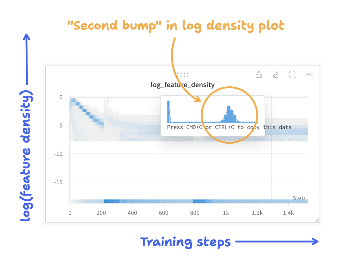
By the end of the training run, notice that there’s a large spike on the left that corresponds to dead or “ultra-rare” features that don’t seem very interpretable, and a smaller bump to the right. That second bump represents a cluster of interpretable features. Anthropic notes similarly shaped feature density plots in their first sparse autoencoder work.
With this setup and knowledge, I swept across the two key hyperparameters, $\lambda$ and learning rate.
I trained these models for 2 epochs with fairly large batch size (512-1024). It seems essential to overtrain these models past when loss plateaus to get good results for interpretability. In retrospect, it’s unclear that repeating training data was helpful, and I would recommend simply collecting more data in the future over training for more than one epoch.
In the end, I could only achieve good results with the 8x-wide SAEs I trained, which are the v6 SAEs I described earlier. I believe other SAEs required quite different hyperparameter choices that I didn’t have time to fully explore.
Automated interpretability
Analogous to OpenAI’s automated interpretability work in Language models can explain neurons in language models, I use GPT-4 to automatically label every feature discovered by these sparse autoencoders, and also to score its own labels for confidence.
This is a two-step process. Prompts used for these steps are documented in the appendix.
-
Labeling with chain-of-thought
I show GPT-4 the top 50 highest-activating example sentences from the training dataset (up to context length limits) for a particular feature, and ask the model to describe the attribute that is most commonly shared across all texts in the list.
-
Normalized aggregate scoring
Both in OpenAI’s work and in this work, GPT-4 biases towards overly general labels, like “Coherent, factual English sentences”. These are not useful, since they are a feature shared by almost any sentence in the dataset. What this usually means is that the particular feature does not have an obvious interpretable explanation.
To filter these out, I added a scoring step. In this step, I ask GPT-4 to rate the fraction of both highly activating and non-activating example sentences which fit the auto-generated label, and take the difference between the two fractions to get a normalized confidence score for how well the label and explanation specifically describe samples from this particular feature.
What results is a dataset of features with the following schema.
type SpectreFeatureSample = {
  text: string;
  act: number;
};

export type SpectreFeature = {
  index: number;      // feature index in the learned dictionary
  label: string;      // short explanation
  attributes: string; // longer explanation, which is often useful
  reasoning: string;  // chain-of-thought/scratchpad output
  confidence: number; // normalized confidence score
  density: number;    // how often is this feature turned on?
  highActSamples: SpectreFeatureSample[];
  lowActSamples: SpectreFeatureSample[];
  vec: number[];      // feature vector in the model's embedding space
};
Results and applications
Understanding embeddings
When ranked by a combination of confidence (GPT-4’s self-assigned interpretability score) and feature density (how frequently does this feature activate in the dataset?), the highest ranking features reliably have obviously human-interpretable explanations, as we can see in the “Feature gallery” section above.
Larger models have more interpretable features when all other hyperparameters are held constant, and larger models also tend to have more specific features. For example:
sm-v6has a Christian religious themes and reflection feature which activates on references to God, the Bible, and Jesus Christ. It also has a related feature that activates on mentions of institutions like the Catholic church.bs-v6has many more feature related to Christianity, including one for mentions of “God” and one about sin and salvation.lg-v6andlg-v6.0have yet more features on this theme, including one specifically about Bible verses and one about eschatological topics like salvation and resurrection.xl-v6features about Christianity are similarly more detailed, including one specifically about apocalyptic themes, and one about interpreting Biblical verses. We also see distinct features for Biblical verses with and without their numbers.
Larger models with higher-dimensional embedding spaces also contain more features for specific words and phrases, in addition to common features about general styles and topics.
It’s also interesting to look at which features activate strongly for a particular text input. For example, on that very sentence, the top features in lg-v6 are:
- Referencing specific objects or conditions, as in “particular”
- Discussion of text formatting
- Expressed interest in further exploration
- High intensity/emotionality, as in “activate strongly”
There’s room for lots of interesting future work studying relationships between features in different embedding spaces, the order in which features are learned through training, when features split as models get larger, what kinds of attributes features tend to represent, and so on.
Text editing in embedding space
Sparse autoencoder features can be used to edit text by manipulating an embedding to make meaningful semantic edits, then reconstructing the embedding back into text with the modification.
This method isn’t yet competitive with prompting larger models for general-purpose text editing. But it works well enough to often make quite precise semantic edits to text, meaning the edit is able to intervene only on the specific attribute of the text we care about, and generally avoid changing other things about the text. This is surprising, because we’re just directly editing numbers in embeddings!
Moreover, the efficacy of latent space intervention like this is further suggestive evidence that features discovered with this method aren’t just showing correlations in the embedding space or doing some rough approximation of clustering, but finding directions that actually represent specific, interpretable units of meaning in the embedding space.
Here are some curated examples of semantic edits on the passage, “This research investigates the future of knowledge representation and creative work aided by machine understanding of language. I prototype software interfaces that help us become clearer thinkers and more prolific dreamers.”
-
Nautical terms and situations = 2.0: Her research involves the exploration of sea and land using the work of computer vision to help ships and crews become more agile and imaginative.
-
Presence of randomness or unpredictability = 1.0: This research investigates the randomization of knowledge resulting from automatic human and computational thinking. She helps collaborators build software tools that are more unpredictable and vividly guessable.
-
Quotation followed by commentary = 1.0: “My research investigates the future of knowledge and human engagement. That enables us to make art better.” I am increasingly passionate about machine learning and creative thinking.
-
Anime or Japanese game references = 1.5: This research investigates how knowledge and intellectual creation is aided by anime and visual art. Shikima hopes to make people more creative and brilliantly code their imaginations.
-
Written in French language = 2.0: La recherche en écriture informatique de la theory des jeux et de la communication faite par la recherche du logiciel. Le savoir accompagners nouveau talents qui improviser dans le creation de la littérature et des leçons réalistes.
Apparently this translates (roughly) to, “Research in computer writing of game theory and communication made by software research. Knowledge to accompany new talents who improvise in the creation of literature and realistic teachings.” Though this is broken French, I was very surprised that even a translation of this precision could be encoded as a single direction in embedding space. When we consider that this model was trained on a dataset that was mostly filtered for English, this is even more surprising!
-
Sweet Treats and Baking = 2.0: This project investigates the creativity of ice cream and sweets made by brilliant writing and delicious smoothies.
Edits can also be composed together. For example, by applying the features for Historical analysis and commentary, Sweet Treats and Baking, and Nautical terms and situations, we can transform the original sentence into this strange combination of ideas.
Her research into the sea and shipwrecks of the Atlantic Ocean enabled the development of modern food and cake decorations and the more sophisticated craft of sailing and vanilla.
Edit methods: balancing steering strength and precision
As a part of this work, I experimented with a few different ways to apply a feature to an embedding to edit text, and found some interesting new approaches that seem to work better in specific situations.
When making semantic edits in latent space, we need to balance two different goals:
- Maximize steering strength. We want to reliably express our desired feature in the model output.
- Minimize interference with other features. We don’t want to accidentally also activate other potentially unrelated features. In other words, we want our edit to be precise.
These goals are at odds with each other. To understand why, we need to think about correlated features.
When we study a dataset of real-world text, we often find distinct features that co-occur often. For example, a feature for “Discussion of economics” is probably likely to co-occur often with a feature for “Mentions of the US government”, since the government often comments on and influences the economy. To take advantage of this fact, an embedding model may learn to point these two distinct features into directions that lightly overlap, because it saves some capacity in the embedding space, and if the model accidentally gets confused, the chances are good that the model’s output will still be coherent.
But this superposition becomes an issue when we want to activate one of these features without the other, because very strongly activating the “Mentions of the US government” may push our embedding far enough along the nearby “Discussion of economics” direction to make a difference in the output. We’ve tried to make a strong edit, and lost precision as a result.
To overcome this tradeoff, I explored a few different “Edit modes” when manipulating embeddings.
Addition. This is the most obvious way to edit embeddings. I simply push the embedding along the feature direction. (Mathematically, I add the feature vector directly to the embedding vector.) This reliably makes strong edits, but also often causes interference between features, resulting in edits where the output looks quite different from my input.
Using the Nautical terms and situations feature edit from above, an edit via addition results in
Her research investigates the development of shipboard knowledge and understanding aided by creative work. This research enabled sailors and engineers to make more fragile and colorful vessels and navigate faster and more dreamily.
The nautical theme is certainly very strongly expressed, but now we’ve lost a lot of the original phrasing and wording.
SAE intervention. In this approach, we try to take advantage of the fact that the sparse autoencoder model has learned how to translate feature activations into embeddings and back. Taking advantage of this, we encode the embedding we want to edit with the encoder of the SAE, modify the value of the feature we care about in-place, and then decode it back into the embedding space, adding any residual that the SAE could not reconstruct as a constant. In theory, because the SAE has learned how to “un-do” some of the interferences between features, this approach should result in “cleaner” edits.
This research venture investigates the representation of human knowledge and navigating under sail assisted by ship work. She designed software and creative ideas to help crews become more proficient and more brilliant navigators.
Word choice and phrasing are closer to the original text, but there’s still a lot that’s changed.
This led me to my final approach, which I call feature gradients. It works like this:
A perfect embedding edit would mean that when we take the edited embedding and put it through the SAE, the resulting feature activation values would exactly equal how much we want each feature to be expressed. What if we used gradient descent to directly optimize for this objective?
When using feature gradients, we:
- First perform the “addition” method to get an approximation of the edited embedding we want.
- Then, we iteratively optimize this approximation through gradient descent, to minimize the difference between (a) the value of
sae.encode(embedding)and (b) the feature activation values we want. Concretely, we do this by minimizing the mean squared error (MSE) between the two values. I’ve found the Adam optimizer with a cosine learning rate annealing schedule to get good results quickly.
You can find a PyTorch implementation of feature gradients in the appendix.
Using feature gradients, we can produce this final edit:
This research lab investigates the development of maritime exploration and art and human knowledge aided by ship building. She trains her crew to become better thinkers and more prolific swimmers.
This version preserves much of the wording and sentence structure from the original text, while expressing the feature very clearly.
Feature gradients is not always the best edit method to use, however. Though I haven’t performed a rigorous study, in my experience making hundreds of edits, addition is most effective if the edit involves steering broad features like topics, voice, or writing style; feature gradients is most effective if the edit is more precise, like adding a mention of a specific word or number. I hypothesize that this is because when editing text to express a broad topic or style, we actually do want to express many related features together, whereas this is undesirable when making edits about phrasing or structure, which are naturally more specific.
Caveats and limitations
TL;DR — this is all building on a relatively new approach to interpretability, and my implementation of the key ideas in this work is a proof of concept more than a rigorous claim about how interpretable embedding spaces are.
- Sparse autoencoders are still a relatively new technique, so current approach isn’t indicative of what’s possible. SAEs are a promising tool for interpreting dense activations of transformers, but definitely just a start.
- All published literature on sparse autoencoders train on much larger datasets than I do (tens of billions of samples vs. ~30M samples repeated twice). I hope to scale up my data, and don’t expect core results to change, but some numbers might.
- My approach to using LLMs to auto-label and auto-evaluate features is less rigorous than OpenAI’s automated interpretability work, trading off rigor for compute (and cost) efficiency. Specifically, my method doesn’t try to simulate feature activations, but instead grades the labels’ ability to uniquely explain highly activating samples. For my purposes (of prototyping interface ideas), this distinction isn’t important, but it’s worth noting.
- I only label features here based on top-activating examples, rather than the full spectrum of activations. This can fall victim to the “interpretability illusion”, wherein feature vectors may stand for more than one human-interpretable attribute, but some get ignored in the labeling process. I hope to address this in a larger-scale follow-up project.
Future work
For me, the most exciting consequence of this work is that it opens up a vast design space of richer more direct interfaces for interaction with foundation models and information. It’ll take me a whole difference piece to explore the interface possibilities I imagine in detail, but I’ll try to share a glimpse here.
Using the two primitives I shared above, (1) decomposing an input into features and (2) making semantic edits, we can assemble ways of interacting with text that look very different from conventional reading and writing. For example, in the prototype below, I can select a specific SAE feature and see a heat map visualization of where in the text that feature was most activated.
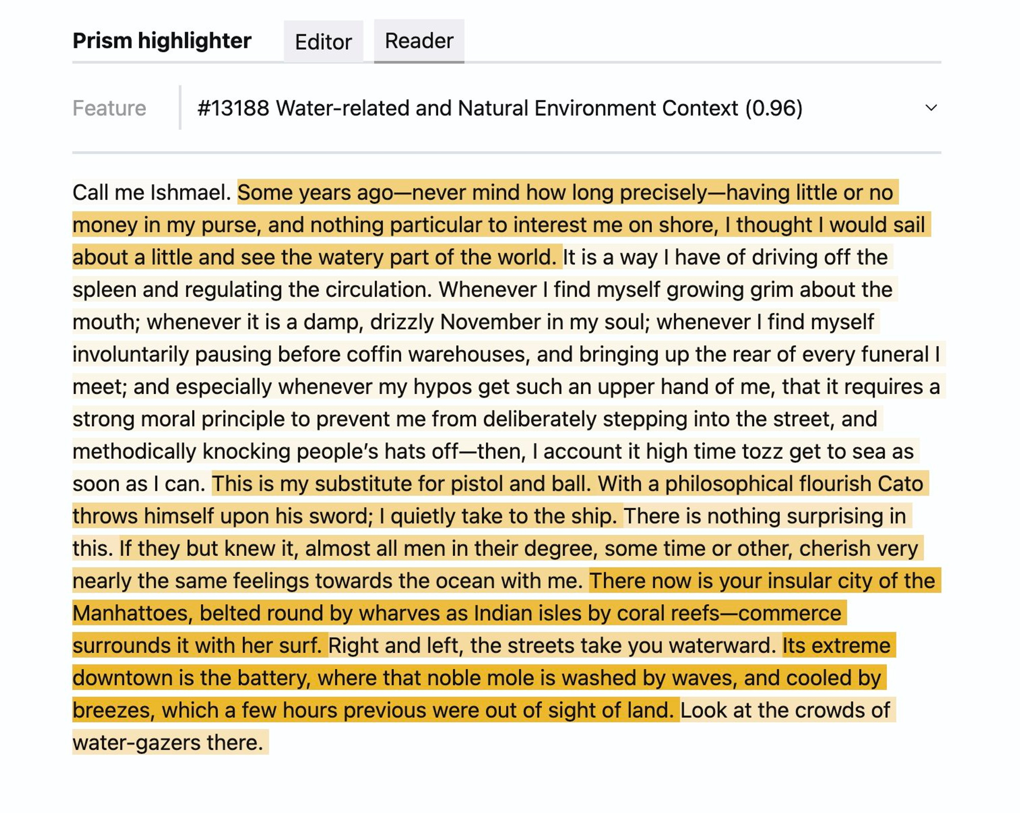
Imagine exploring much longer documents, or even vast collections of documents, by visualizing feature maps like this at a bird’s eye view across the whole set at once rather than reading and tagging each document one by one.
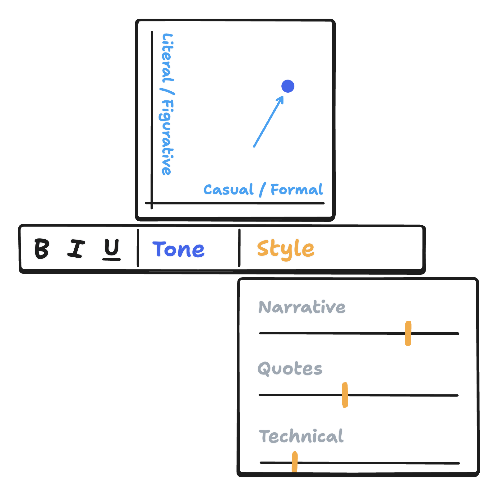
On the editing side, there are many interesting ways we could surface precise semantic edits in a writing tool. Here, for example, we can imagine a text editing toolbar that doesn’t just expose formatting controls like bold, italic, and underline, but also continuous controls for tone, style, structure, and depth of material.
In the future, it may also be possible to “copy style” of a piece of writing or image and “paste” those same stylistic features onto another piece of media, the same way we copy and paste formatting. In general, as our understanding of latent spaces of foundation models improve, we’ll be able to treat elements of semantics, style, and high-level structure as just another kind of formatting in creative applications.
There is also no shortage of areas of improvement beyond interfaces.
Most urgent for me is scaling SAEs to more production-scale models, and generalizing these techniques to models of other modalities like image, audio, and video. In particular, I’m currently working on extending this work to:
- A production-grade open-weights language model like Llama 3 8B
- A production-grade multimodal embedding model like
nomic-embed-v1.5for both text and images - OpenAI’s CLIP text-image embedding model (some concurrent related work here from Fry, 2024 and Daujotas, 2024)
- Code embedding and generation models
The core science behind SAEs and dictionary learning can also improve a lot, including advancements in SAE architecture and training recipes. Major AI labs with alignment teams like DeepMind and Anthropic are making major strides on this front. A recent example is gated sparse autoencoders, which improve upon the state-of-the-art to yield cleaner, more interpretable features.
Lastly, everyone working with SAEs would benefit from a deeper understanding of how features and feature spaces relate to each other across different models trained over different datasets, trained with different architectures, or trained on different modalities.
Looking back, looking forward
Since I first began researching how to build latent space-based information interfaces in 2022, it was clear to me that model-learned representations were key to a big step forward in how we interact with knowledge and media. To borrow some ideas from Using Artificial Intelligence to Augment Human Intelligence (one of whose authors now leads Anthropic’s interpretability research), machine learning gives us a way to automatically discover useful abstractions and concepts from data. If only we could find a way to mine these models for the patterns they’ve learned and then interact with them in intuitive ways, this would open up a lot of new insight and understanding about our world.
While iterating on design prototypes in mid 2022, I hit a big roadblock. Though I had built many ways to work with embeddings in relation to each other, like clustering them and finding interpolations between them, to make embeddings truly useful, I felt I needed some way to know what an embedding actually represented. What does it mean that this embedding has a “0.8” where that embedding has a “0.3”? Without a way to give meaning to specific numbers, embedding spaces were glorified ranking algorithms. This problem of interpretability, this understanding gap, felt like a fundamental problem preventing interface innovation in this space.
I wrote at the time:
I’ve been researching how we could give humans the ability manipulate embeddings in the latent space of sentences and paragraphs, to be able to interpolate between ideas or drag sentences across spaces of meaning. The primary interface challenge here is one of dimensionality: the “space of meaning” that large language models construct in training is hundreds and thousands of dimensions large, and humans struggle to navigate spaces more than 3-4 dimensions deep. What visual and sensory tricks can we use to coax our visual-perceptual systems to understand and manipulate objects in higher dimensions?
This core challenge of dimensionality, I think, still remains. In some ways, we’re now finding the problem to be much worse, because instead of working with embedding spaces of a few hundred dimensions, it turns out we ought to work with feature spaces of millions or even billions of concepts. But rendering embeddings legible, giving meaning to specific numbers and locations and directions in latent space, is a meaningful step forward, and I’m incredibly excited to explore both the technical and interface design advancements that are sure to come as we push our understanding of neural networks even further.
Appendix
I. Automated interpretability prompts
These are formatted a little oddly because they’re excerpted from a Notion-internal prompt engineering framework.
Here’s the prompt for generating feature labels and explanations.
`What are the attributes that texts within <positive-samples></positive-samples> share, that are not shared by those in <negative-samples></negative-samples>?`,
``,
`<positive-samples>${
  formatSamples(highActSamples, { mode: "tokens", max: 3000 })
}</positive-samples>`,
`<negative-samples>${
  formatSamples(lowActSamples, { mode: "tokens", max: 3000 })
}</negative-samples>`,
``,
`Before you respond, try to identify the most specific attribute that are shared by all positive samples, and none of the negative samples. The more specific the better, as long as only all positive samples share that same attribute.`,
``,
`First, describe your reasoning in <reasoning></reasoning> tags.`,
`Then, describe the shared attributes in <attributes></attributes> tags. Within these tags, do not reference any tags or the words "positive" or "negative"; simply refer to samples as "the samples".`,
`Finally, within <label></label> tags, write a short, 4-8 word label for this attribute in sentence case.`,
Here’s the prompt used to compute the normalized aggregate score for each feature’s explanation.
`I have a dataset of text snippets:`,
`<samples>${
  formatSamples(samples, { mode: "tokens", max: 4000 })
}</samples>`,
``,
`What percent of the samples fit the attribute described below?`,
`<attribute>${attributes}</attribute>`,
``,
`Give your answer as an integer between 0 and 100 inclusive, enclosed in <percent></percent> tags, as in <percent>NN</percent>.`,
`Do not include the percent sign in your response; include only the number itself.`,
II. Feature gradients implementation
Note: here, spectre is an implementation of sparse autoencoders in my research codebase.
def dictgrad(
    spectre: nn.Module,
    x: torch.FloatTensor,
    f: torch.FloatTensor,
    original_features: torch.FloatTensor,
    # method-specific config
    steps: int = 500,
    **kwargs,
) -> torch.FloatTensor:
    # "Reference" is the text, latent, and feature dictionary we want to edit.
    reference_latent = x.clone().detach().requires_grad_(False)
    reference_features = original_features.clone().detach().requires_grad_(False)

    # Initialize with the "addition" edit method.
    latent = addition(spectre, x, f, original_features, **kwargs).clone().detach().requires_grad_(True)

    # Adam optimizer with cosine annealing works faster than SGD, with minimal
    # loss in performance.
    optim = torch.optim.AdamW([latent], lr=0.001, betas=(0.9, 0.999), eps=1e-08, weight_decay=0.0)
    optim.zero_grad()
    scheduler = torch.optim.lr_scheduler.CosineAnnealingLR(optim, steps, eta_min=0, last_epoch=-1)

    # Gradient descent: we optimize MSE loss to our desired feature dictionary.
    for step in range(steps):
        features = spectre.encode(latent)
        loss = F.mse_loss(features, reference_features)
        loss.backward()

        optim.step()
        optim.zero_grad()
        scheduler.step()
    return latent
III. FAQs
Why interpret embeddings and not language models?
Many other research groups are applying this technique to autoregressive language models. Why embeddings?
I worked on applying SAEs to embeddings because:
- From the beginning, my aim is to build tools that work with information in units that are natural for humans. Humans work with thought at the level of sentences and paragraphs, not sub-word tokens. It seemed useful to work with a model that represented information at the same altitude.
- I think embeddings are interesting as a kind of “storage at rest” form of how models represent information, rather than “storage in transit” format, which is what LLMs contain when it’s generating text.
- Nobody else was applying SAEs to embeddings at the time (December 2023).
The basics of the technique transfer well between the two settings, so I plan on eventually returning to autoregressive language models as well.
I see these results are using a custom embedding model. Does this generalize to other widely used embedding models?
I haven’t tried this, so can’t say with 100% confidence, but based on my experiments mapping this model’s embedding space to that of text-embedding-ada-002 from OpenAI, the technique should transfer very well to any reasonably good embedding model. One of my follow-up projects is to validate this claim.
Much gratitude to the many people who offered ideas, advice, resources, and encouragement through this project, including Gytis Daujotas, Matthew Siu, Dan Shipper, Theo Bleier, Maya Bakir, Betaworks, and others.
← Personalization, measuring with taste, and intrinsic interfaces
I share new posts on my newsletter. If you liked this one, you should consider joining the list.
Have a comment or response? You can email me.